Classifying data with decision trees 01 Jul 2018

What is a decision tree?

Supposedly you want to sort three values, A, B, and C. But you want to do this in an intuitive way, such that a 5-year-old would understand your process. What are you going to do? Get a 5-year-old and have them sort those values. They are going to look at the three values and decide to divide them unconsciously in smaller subproblems. First, they wonder if A is smaller than B. Then, they want to see if B is smaller than C. If A < B and B < C, then they conclude that A < B < C. But, if B is not smaller than C, then a third question comes to mind, is A < C. The kid gets lost with all those different solutions and decides to keep track of them by writing them down. He draws a node for each question and an edge for each answer. Unconsciously he draws a solution that might look like the one Figure 1.

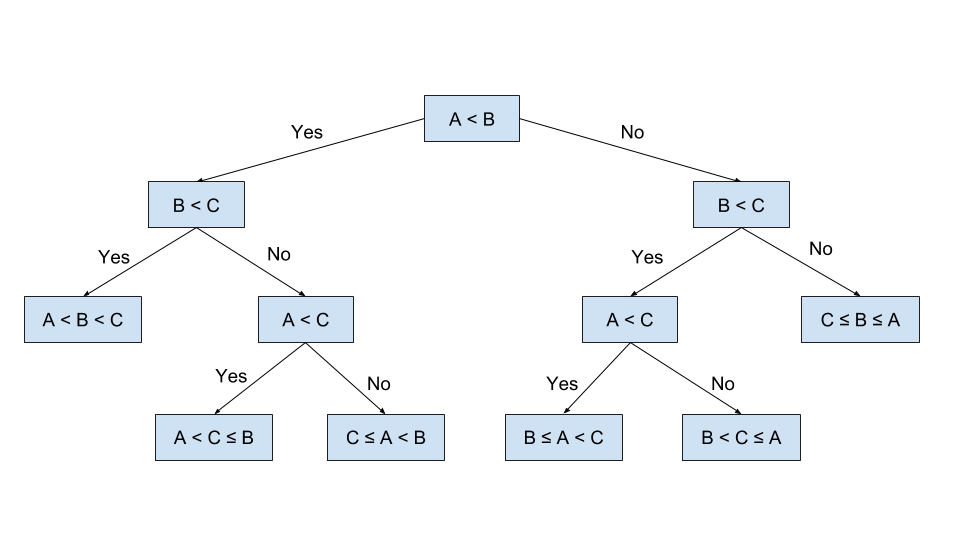
With no further knowledge about trees or what they are representing, the kid has created his first decision tree and has given us an intuitive way to approach the problem of sorting those three values. An astute reader who has knowledge of computer science and algorithms may even observe that the tree in Figure 1 represents the insertion sort algorithm for three values. But, that is inconsequential to our kid, what we wanted was to develop a simple and intuitive algorithm to sort three values, an algorithm that could be extended to N values if we would like so.
Having in mind the previous example, now we are ready to give a technical non-technical definition of a decision tree. A decision tree is basically a binary (or n-ary) tree flowchart where each node splits a group of observations according to some feature variable. The goal of a decision tree is to split your data into groups such that every element in one group belongs to the same category. A decision tree is a type of non-parametric supervised learning algorithm that is used in both classification and regression problems. It is a representation of predictive modelling used in statistics, data mining and machine learning.
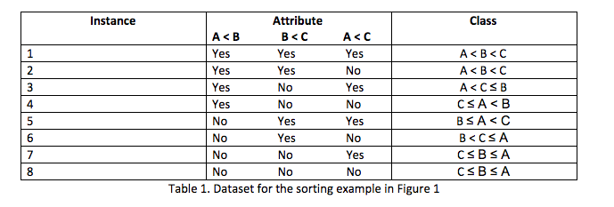
In supervised learning problems, we start with a dataset containing training examples with associated correct labels. This input is called the set of instances (e.g. rows, examples or observations). Each of those instances is described by a set of attributes (i.e. columns), which are assumed to be either nominal or numeric, and a label which is called a class (in case of a classification task). Going back to the task of sorting three values: each decision in our tree becomes an attribute (all binary relations), all leaves of the tree are classes, while each row in Table 1 represents an instance of the dataset. The algorithm will then learn the relationship between the instances and the classes and apply that relationship to further classify completely new instances that the machine hasn’t seen before.

Mathematical background and general algorithm

Now that we have an intuitive knowledge about decision trees and how they are representing data, we can give a mathematical formulation for them.
Given training vectors , i =1, …, l and a label vector , a decision tree recursively partitions the space such that the samples with the same labels are grouped together.
If we let the data at node m be represented by the set Q, then for each candidate split Θ = (j, tm) consisting of a feature j and the threshold tm, partition the data into Qleft(Θ) and Qright(Θ) subsets, where:
Qleft(Θ) = { (x, y) | xj ≤ tm} Qright(Θ) = Q – Qleft(Θ)
Algorithms for constructing decision trees usually work top-down, by choosing a variable at each step that best splits the set of items. There are different algorithms for implementing decision trees, and those algorithms use different metrics to describe the “best” criterion for splitting. In general, those criteria measure the homogeneity of the target variable within the subsets. But, regardless of those criteria we could devise a general algorithm for a decision tree as in Listing 1.

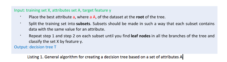
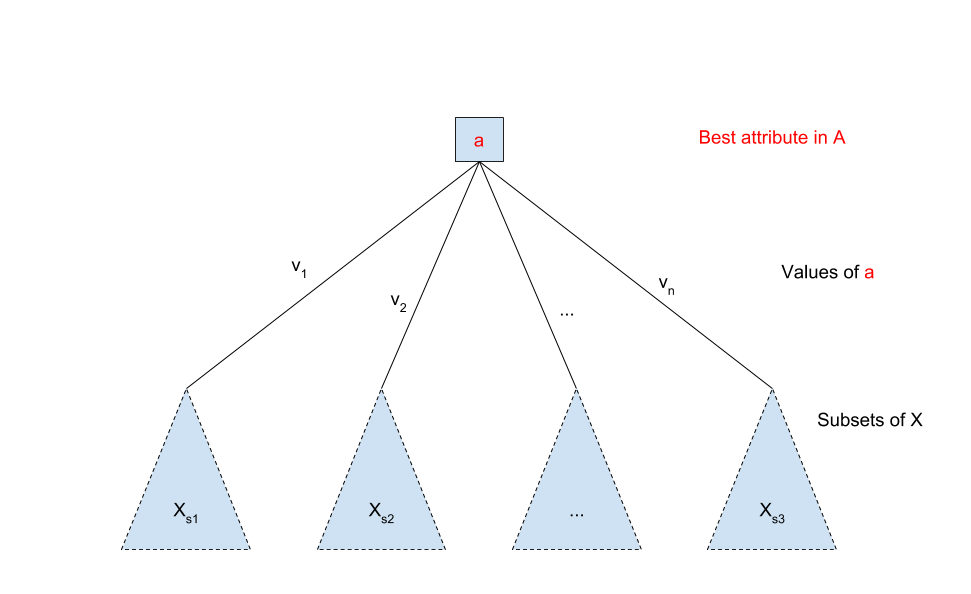
To make it clear how this algorithm works, we can look at a simplified run through for the first loop. We first select the best attribute, a, from the set of attributes A. Based on the values of a we split the training set X into subsets, values v1 to vn , each of those Xs1 to Xsn subsets represent now the new training set and we are calling the algorithm recursively on them. We stop when we find leaf nodes or when we have reached a user defined stopping criteria. We can see the results of the construction of the tree after one step through the loop in Figure 2.

Decision trees can be used for both classification and regression, as we stated before, but even though they are very similar to each other there are a couple of differences between the two of them. In general, classification trees are used when the dependent variable is categorical (either True/False, Male/Female etc.), and regression trees are used when the dependent variable is continuous. In this case of regression trees, the value obtained by terminal nodes in the training data is the mean response of observation falling in that region (so, if an unseen data observation falls in that region, the prediction will be made based on the mean value). Both regression and classification trees divide the space into distinct and non-overlapping regions, as we could see from Figure 2. The splitting process finishes when the stopping criteria is reached, this results in fully grown trees that might overfit the data (the function is too closely fit to the training dataset). This can be mitigated with “pruning”.

Splitting choice

How does a tree decide where to split? There are multiple algorithms to decide to split a node in two or more sub-nodes, and those algorithms are different for classification and regression trees. The goal of a splitting choice is to increase the homogeneity of the sub-nodes, meaning that the purity of the node increases in respect to the target variable. Thus, a decision tree splits a node on all the available variables and then from the available splits selects the one that results in the most homogeneous sub-nodes, it’s a greedy approach.
Two of the most commonly used methods in decision tree algorithms are Gini Index and Reduction in variance. The former algorithm deals with categorical attributes and classification trees, the later deals with continuous attributes and regression trees.
The Gini Index method works with categorical target variables as “Success” or “Failure”, and it performs only binary splits. In this algorithm if we select two items from a population at random then they must be of the same class and probability for this is 1 if the population is pure. The rule is that the higher the value of the Gini index then the higher the homogeneity. This method is employed by the CART algorithm (Classification and Regression Tree). A Gini score gives an idea of how good a split is by how mixed the classes are in the two groups created by the split. A perfect separation results in a Gini score of 0, whereas the worst case split that results in 50/50 classes in each group result in a Gini score of 0.5 (for a two-class problem).
The Reduction in variance method is used for continuous target variables in regression problems. It uses the standard formula of variance to choose the best split: Variance = Σ( X – X’)2 / n (where X is the actual value in the data set, X’ is the mean of the values in the data set, and n is the number of values). The criteria to split the population is the split with lower variance is the one that is always chosen.

Practical application – IRIS data set

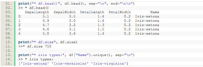
To make things clearer we are going to run a classifier on the IRIS dataset in python and see how decision trees are working on a live example. The dataset is available for loading from the Sklearn library in Python, or you could load it manually after downloading the file from [1]. The dataset consists of various measurements for various types of irises. If we do a little exploration of the dataset, we can see the attributes of the data in the form of sepal length and width, and petal length and width, as well as the iris types (Iris-setosa, Iris-versicolor, and Iris-virginica). This can be seen in Listing 2.

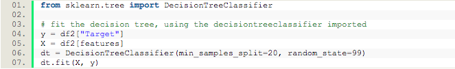
From this information, we can talk about our goal: to predict Name (or, type of iris) given the features SepalLength, SepalWidth, PetalLength and PetalWidth. In order to be able to pass this dataset into a classifier we need to map the Name attribute to a value, so we map Iris-setosa to 0, Iris-versicolor to 1, and Iris-virginica to 2. Now we can use the DecisionTreeClassifier function from the Sklearn library to fit the on the data. Sklearn will generate a decision tree for the IRIS dataset using an optimized version of the CART algorithm when you run the code in Listing 3. Remember that the CART algorithm uses the Gini Index by default as a method to decide the splits. The decision tree is initialized with two parameters: min_samples_split=20 which tells us that a node requires 20 samples in order for to be split and random_state=99 to seed the random number generator that the classifier uses.

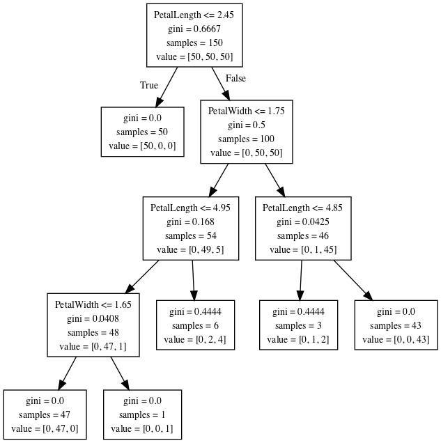
A visualization of the tree can be seen in Figure 3. All the data instances (all the rows) start in a single bin, at the root of the tree. All the features of the data (SepalLength, SepalWidth, PetalLength and PetalWidth) are considered in order to find the best split using the Gini Index. At the root of the tree the most informative condition is PetalLength ≤ 2.45. If this condition is true then the left branch is taken and this gives us a bin of 50 samples, with the target value 0. From the earlier mapping of the Names to the values, value 0 corresponds to Iris-setosa. The other 100 values go to the right bin and the splitting process continues. The process stops either when the split creates a bin with only one class, or the bin has less than 20 samples.

Conclusion

There are a couple of advantages of deploying Decision Trees in practice. They are self-explanatory and can be easily converted into a set of rules, which is easy and fast to interpret, understand, and implement. (e.g. if you have a path from the root to the tree then that’s your resulting classification given by the leaf node) Decision trees are versatile, they can handle both nominal and numeric data, are non-parametric which means that they have no assumptions about the space distribution and the classifier structure, and they are capable of handling data sets with missing values.
At the same time, we pay for the ease of use and understanding in terms of oversensitivity to the training set, to irrelevant attributes and to noise. Decision Trees tend to perform well if we have a few highly relevant attributes (they use divide and conquer on those attributes), but they perform poorly when many complex interactions are present.
That being said, Decision Trees have their uses and tree based models are known to provide good performance in the family of machine learning algorithms. Even though the splitting decision that the tree makes at each node is optimized for the data set it is fit to and will rarely generalize well to other data, we can generate huge numbers of those trees, tuned in different ways, and combine their predictions to create a more robust model.

Bibliography:
[1] https://raw.githubusercontent.com/pydata/pandas/master/pandas/tests/data/iris.csv
[2] http://scikit-learn.org/stable/modules/tree.html#classification

This work has been published in the ACM XRDS magazine, the Summer 2018 issue.

Let me know what you think!