Applying Data Science for Anomaly and Change Point Detection 20 Sep 2018

What do we mean when we say that we are trying to find anomalies in a data set? What are anomalies? How can we define a point in the data starting with the behavior of the data is becoming anomalous? Those are the questions that we are going to try to answer in this introductory article about anomaly detection and with the help of a running example using network data we are going to devise a couple of very simple algorithms for anomaly detection.

What are anomalies?

Anomaly detection refers to the problem of finding patterns in data that are not aligned with the expected behavior. We are looking for outliers, exceptions or discordant observations that when we are viewing the entire set of data look out of place.

Anomalies are patterns in the data that do not conform to a well-defined notion of normal behavior. In Figure 1 we can observe a series of two dimensional points that are being categorized in a couple of regions that form two clusters C1 and C2 . The points that are far away from those regions, like O1 and O2 are considered outliers since they do not align to the normal region.

Anomalies can be broadly categorized as: point anomalies - when a single instance of data is anomalous if it’s too far off from the rest, like O1 and O2 from Figure 1. Point anomalies can be used to detect credit card fraud based on amount spent. Contextual anomalies where the abnormality is context specific, those are very common in time-series data: anomalies in network traffic patterns - based on the throughput a network has at some point in comparison to an usual, it might be usual that there is a high traffic during the early morning in USA and a slow down during the lunch hours but not vice-versa. Collective anomalies are the type of anomalies that are being detected with the use of a set of data instances. For example on a Linux machine the following events might appear: http-web, buffer-overflow, http-web, http-web, smtp-mail, ftp, http-web, ssh, smtp-mail, http-web, ssh, buffer-overflow, ftp, http-web, ftp, smtp-mail,http-web … the events in bold are not an anomaly taken individually but in taken in the collectively with the ftp_transfer event might signal a potential cyber-attack, someone exploited a buffer overflow vulnerability and is now copying data from a remote machine to the local host.

The process of anomaly detection has a couple of important challenges. Since we want to discover a pattern that does not conform to normal expected behavior in the data a first step into the anomaly detection process is to first define a normal baseline behavior and then declare any observations that are not aligned with this normal behavior as anomalies. But, defining a region that covers all normal behavior is very difficult, especially when the boundary between normal and abnormal behavior is hard to define. On top of that, in many domains what is classified as normal behavior keeps evolving so the model needs to evolve as well. Speaking of model, usually the labeled data for training/validating the model is not readily available and in most cases contains noise that might be similar to the anomalies that we want to detect.

Considering those challenges the problem of anomaly detection in a general form is usually not easy to solve, that’s why there are specific variations of the problem that are being solved keeping in mind the nature of the data, the availability of labeled and unlabeled data and the types of anomalies that are trying to be detected.

Anomaly detection techniques very short overview

When it comes to classifying the anomaly detection techniques there are a couple of attributes over which we can classify them. Based on the extend on which labels are available in the data we can apply: supervised anomaly detection techniques which assume the availability of a data set that has labeled instances for normal as well as abnormal classes. Semi-supervised anomaly detection techniques that operate in a semi-supervised mode, in which the data has labels only for the normal classes. And finally, unsupervised anomaly detection techniques that do not require training data and are most widely used.

Another way to classify the anomaly detection techniques is based on the underlying algorithm they are using. Considering that we have: classification based techniques where classification is used to learn a model from a set of labeled data instances (training set) and then classify a test instance into one of the instances (testing). In this category we have Neural Network Based, Bayes Based, Rule Based and Support Vector Machine Based algorithms. Clustering based anomaly detection techniques is used to group similar data into clusters, with the assumption that normal data belongs to a cluster while anomalous data doesn’t belong to any cluster. Statistical anomaly detection techniques are techniques that assume that an anomaly is “an observation that is suspected of being partially or wholly irrelevant because it is not generated by the stochastic model assumed” [4]. The underlying principle is that normal data points occur in high probability regions of a stochastic model, while anomalies occur in low probability regions of the said model.

Next we are going to get a more in detail look at the Statistical anomaly detection techniques, specifically the parametric and non-parametric ones, and later on we are going to do see the two methods in action running an example on some network data.

Statistical anomaly detection techniques

As we have mentioned before, when we are using statistical anomaly detection techniques we are looking for normal data instances that are occurring in high probability regions of a stochastic model, whole anomalies occur in the low probability regions of the said stochastic model. How does a statistical technique work? It fits a statistical model for normal behavior to the given data and then it applies a statistical inference test to determine if an unseen instance belongs to this model or not. If an unseen instance has a low probability of being generated from the learned model, based on the applied statistic, then that instance is an anomaly.

There are two types of statistical techniques, parametric and non-parametric ones. The main difference between the two of them is that parametric techniques assume the knowledge of the underlying distribution and estimate the parameters from the given data [3], while the non-parametric ones don’t assume any knowledge about the distribution of the underlying data. We are going to see a comparison of the two models, by running a parametric technique - the Gaussian Model algorithm - and a non-parametric one - the CUSUM algorithm - on a data set and try to detect the anomalies and the points of change in the trends underlying the data. We are going to find outliers in computer servers network data.

Anomaly detection using network data

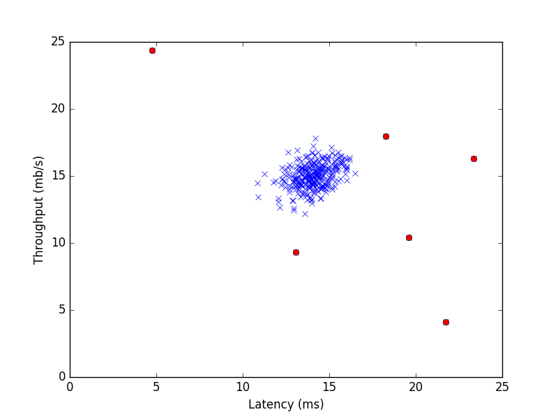
The data we are using to illustrate this example is quite simple, it only has two features: i) throughput in mb/s and ii) latency in ms of response for each server. The data will be broken down in 2 sets, the training set and the test set, each of them with around 300 samples (a very small data set) [2]. Since we are dealing with a limited number of features here, two - throughput and latency, plotting helps to visualize the outliers. For higher dimensional data this is in most cases not possible. We can see the plotted data in Figure 2.

The Gaussian Model Algorithm assumes that the data is generated from a Gaussian distribution. The parameters are estimated using Maximum Likelihood Estimate [1]. The distance between a data instance and the estimated mean is the anomaly score for that instance. To be able to determine the anomalies we apply a threshold to the anomaly scores.

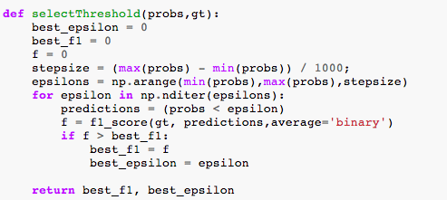
This model is used to learn an underlying pattern of the dataset with the hope that our features follow the Gaussian distribution. We find data points with very low probabilities of being normal and thus with high probability of being outliers. For training set, we learn the gaussian distribution of each feature for which mean and variance of features are required. To find the optimal value of the threshold we try different values in a range of learned probabilities on a cross-validation set. The f-score or the measure of the test’s accuracy is being calculated for predicted anomalies based on the ground truth data available. In Listing 1 we can see the threshold function that we are going to utilize for selecting the anomalies.

We can visualize the highlighted outliers in Figure 3, we can see that our assumption that the initial data was having an underlying Gaussian distribution was correct. But the method is not very precise, since many of the close points to the main cluster were not detected as outliers, though in some situations they might be.

CUSUM Algorithm is one of the classic techniques used for detecting point changes in data and more recently for detecting anomalies. The implementation for the CUSUM algorithm varies, one form of it involves the calculation of the cumulative sum of positive and negative changes (gt+, gt-) in the data and comparing to a threshold. If the threshold is exceeded then a change must have occurred and the cumulative sum is restarted from 0. Of course, the data might present a slow drift either upwards or downwards and that might be detected as a change. To avoid that the algorithm can be tuned with a drift parameter. The proper working of the algorithm depends on those two parameters: threshold and drift. So, properly tuning those is desirable. The literature recommends to start with a very high threshold, choose drift as half of the expected change in the data, then set the threshold in such a way that the number of false alarms (false changes in the data) is obtained.

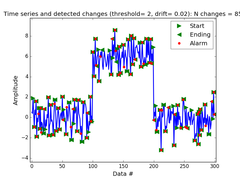
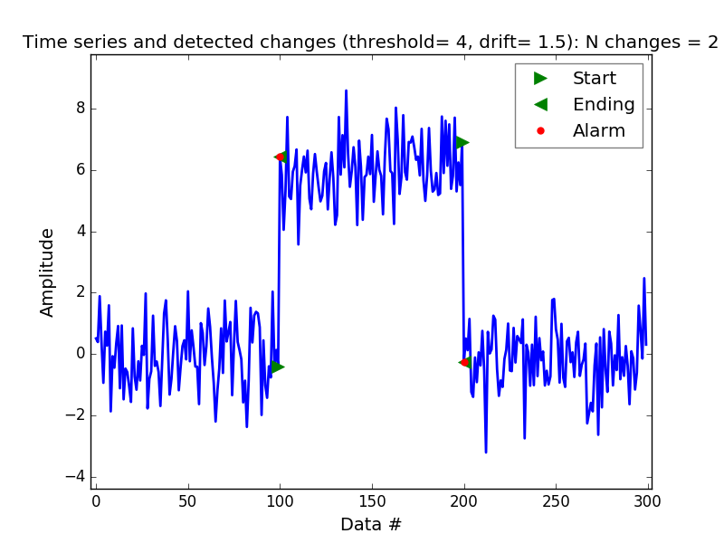
We are going to try to detect the points of change and anomalies on the same data set from before, we are going to use the latency column as the time series on top of which we are going to run the CUSUM algorithm. And to illustrate the point of tuning the threshold and drift parameters properly we are going to have two runs of the algorithm. One, very bad, where almost every point in the series is considered an anomaly and a change point. This can be observed in Figure 4 where we have a threshold of 2 and a very low drift parameter equal to 1.5 . On the other hand in Figure 5 we can observe that by adjusting the threshold, this time it has a value of 4, and the drift parameter, we are allowing the trend to move either way by 1.5, we are obtaining a way better outcome.

Conclusion

There is a huge number of applications for anomaly detection techniques. Each one of those applications come with its own set of challenges and there is no one size fits all model that would work for all of those problems. Some of the applications and their particularities are: intrusion detection systems where the biggest challenge is the huge amount of data so we need methods that are computationally efficient, fraud detection and detection of criminal activities occurring in banks, credit card companies, insurance systems and so on. This comes with time constraints, the sooner the fraudulent transactions are being detected the better. And as we have seen, there is an application of anomaly detection in computer networks as well, in detecting changes in throughput and quality of service offered by the network.
Each of the techniques we overviewed in this article have their own strengths and weaknesses, and of course there are many more techniques than those we have overviewed here. The main getaway from this is that it’s important to know which anomaly detection technique is best suited to a given problem, and even though given the complexity of the problem space it is not feasible to provide such an understanding for every anomaly detection problem we can at least get a general intuition about them.

Bibliography:
[1] https://en.wikipedia.org/wiki/Maximum_likelihood_estimation
[2] https://github.com/elf11/XRDS/blob/master/tr_server_data.csv
[3] https://academiccommons.columbia.edu/download/fedora_content/download/ac:125814/content/anomaly-icml00.pdf
[4] http://amstat.tandfonline.com/doi/pdf/10.1080/00401706.1960.10489888

This work has been published in the ACM XRDS magazine, the Fall 2018 issue.

Let me know what you think!